Krylov Subspace Methods

Lecture notes · about 15 min · last revised 2026-08-17

1 Krylov subspaces

When a matrix is available only as an operator — a routine that returns Av — direct factorizations are out of reach. The only information one can gather is a sequence of matrix–vector products starting from a right-hand side b, and the natural space they span is

Definition

The Krylov subspace generated by A and b is

K k (A, b) = span{ b, Ab, A 2 b, \dots, A k-1 b }.

The name is honest history: A. N. Krylov used exactly such a chain in 1931 to hand-compute the oscillation frequencies of a ship. By Cayley–Hamilton the sequence stalls at the degree of the minimal polynomial — and if that degree is small, the exact solution A⁻¹b already lies in a modest Krylov space. Sparse systems that arise from discretized PDEs and networks are frequently of exactly this kind.

2 Arnoldi and Lanczos

Orthonormalizing the chain gives the Arnoldi process: a sequence q₁, q₂, … with

A Q k = Q k H k + h k+1,k q k+1 e k T,

where H_k is upper Hessenberg. When A is symmetric, H_k collapses to tridiagonal — three-term recurrences, hence the Lanczos process, whose cost per step is one matrix–vector product and O(n) work. The eigenvalues of the small H_k (Ritz values) approximate the extremal eigenvalues of A astonishingly quickly, which is why Lanczos remains the workhorse for large symmetric eigenproblems.

3 Conjugate gradients

For symmetric positive definite systems, Hestenes and Stiefel (1952) turned the Lanczos process into a direct solver that behaves like an iterative one: minimize the A-norm of the error over each Krylov space, in closed form.

r₀ = b − Ax₀;  p₀ = r₀
for k = 0, 1, 2, …
    α   = (rᵣᵗ rᵣ) / (pᵣᵗ A pᵣ)
    xᵣ́₁ = xᵣ + α pᵣ
    rᵣ́₁ = rᵣ − α A pᵣ
    β   = (rᵣ́₁ᵗ rᵣ́₁) / (rᵣᵗ rᵣ)
    pᵣ́₁ = rᵣ́₁ + β pᵣ   until ‖rᵣ́₁‖ small

Two scalar axpys and one matrix–vector product per step; no factorization ever touches A. Conjugate directions are mutually A-orthogonal, and after at most n steps the exact solution appears (in exact arithmetic). In practice one stops tens or hundreds of steps early.

4 Convergence theory

Bound (CG error)

In exact arithmetic,

‖x k - x*‖ A \leq 2 ρ k ‖x 0 - x*‖ A, ρ = (\sqrtκ - 1) / (\sqrtκ + 1),

where κ = κ(A) is the condition number.

The bound is conservative — CG converges according to the distribution of eigenvalues, not merely the ratio λ_max/λ_min; isolated extreme eigenvalues are deflated after a few steps. Non SPD systems lose the minimization structure entirely: for indefinite symmetric systems MINRES replaces CG, and for general systems GMRES works but its convergence depends on the whole spectrum and the eigenvectors — see the eigenvalue scatter in the spectral-theory note for a picture of the worst case.

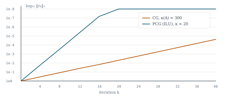
Log-scale convergence of CG versus preconditioned CG

Figure 1. Illustrative residual histories on a model Poisson-type problem: plain CG with κ ≈ 300 against ILU-preconditioned CG with an effective κ ≈ 20.

5 GMRES

The GMRES algorithm (Saad–Schultz, 1986) minimizes the residual norm over x₀ + K_k for arbitrary A. Each step appends a column to the Arnoldi factorization and solves a small least-squares problem with a Givens-updated QR factorization. The cost — one vector more of storage and O(k) work per step — grows linearly, so restarted variants (GMRES(m)) cap memory at the price of possibly stagnating convergence. RULES of thumb: nonzero/repeated eigenvalues clustered away from zero mean fast convergence; eigenvalues surrounding the origin in a disk mean trouble.

6 Preconditioning

Everything above solves the system M⁻¹A x = M⁻¹b just as happily, for any easily inverted M. The art of numerical linear algebra is choosing M ≈ A so that M⁻¹A has a friendlier spectrum:

Jacobi / diagonal: scales row norms; cheap first aid.
Incomplete factorizations (ILU): drop small entries during a truncated Gaussian elimination.
Sparse approximate inverse (SPAI): build M directly, robust in parallel.
Geometric or algebraic multigrid (AMG): for elliptic problems, the only asymptotically optimal choice; roughly O(n) total work.

Modern large-scale solvers — PETSc, Trilinos, hypre — are at heart vast, well-engineered libraries for picking and composing these Ms; see the resources page.

References

M. R. Hestenes, E. Stiefel, "Methods of conjugate gradients for solving linear systems," J. Res. NBS 49 (1952), 409–436.
C. C. Paige, M. A. Saunders, "Solution of sparse indefinite systems of linear equations," SIAM J. Numer. Anal. 12 (1975), 617–629.
Y. Saad, M. H. Schultz, "GMRES: a generalized minimal residual algorithm for solving nonsymmetric linear systems," SIAM J. Sci. Stat. Comput. 7 (1986), 856–869.
Y. Saad, Iterative Methods for Sparse Linear Systems, 2nd ed., SIAM, 2003.