Randomized Matrix Approximation

Research notes · about 16 min · last revised 2026-11-09

1 Why low rank is everywhere

Matrices distilled from the physical world — discretized operators, image stacks, term-document counts, recommendation feedback — rarely have numerically full rank. Their singular values decay, and decay fast, which by the Eckart–Young theorem means a rank-k surrogate with small k already carries nearly all the information.

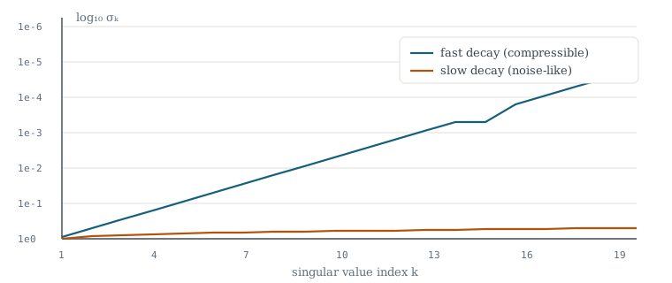
Fast versus slow singular value decay on a log scale

Figure 1. Two singular value spectra on a log scale. Fast decay (blue) makes the matrix compressible; slow decay (amber) is essentially noise-like and resists approximation.

Classical dense SVD algorithms cost O(mn·min(m,n)) — and they insist on touching every entry, even though the answer is determined mostly by a low-dimensional subspace. The randomized paradigm asks a cheaper question first: can we find the dominant subspace with a handful of random sketches, and only then run an expensive deterministic procedure on a much smaller matrix?

2 The randomized range finder

The core algorithm is four lines. Fix a target rank k and an oversampling parameter p (say p = 10):

draw an n×(k+p) standard Gaussian matrix Ω
form the sketch Y = A Ω                      (k+p matrix–vector products)
orthonormalize: Q = orth(Y)
return Q   — approximately, range(Aᵣ) ≈ range(Q)

The intuition is sampling theory in disguise: a Gaussian random combination of the columns of A almost surely retains every direction the matrix cares about, with weights proportional to that direction's energy. Any subspace that captures significant singular energy is likely to appear in the sketch; directions with tiny σ_i may be lost, but by definition they barely matter. The deterministic postprocessing — project, form the small Q^TA, and take its SVD — costs O(mn(k+p)), a factor min(m,n)/(k+p) cheaper than the full decomposition.

3 Oversampling and power iteration

Two knobs control quality. Oversampling (p extra samples) protects against the randomness of the last few captured singular directions — the tail is where sketch variance concentrates. Power iteration replaces Y = AΩ by Y = (AA^T)^qAΩ, which sharpens the spectrum by raising each singular value to the power 2q+1: gaps that were modest become decisive. In practice q = 1 or 2 suffices, provided each application is re-orthonormalized to fight rounding error — otherwise the scheme quietly degenerates toward the dominant singular triplet.

4 Error guarantees

The advertised accuracy is not folklore. For the prototype estimator the average-case analysis is exact.

Theorem (Halko–Martinsson–Tropp, 2011)

Let Q be the output of the range finder with target k and oversampling p ≥ 2. Then for a fixed Gaussian Ω in expectation, and with high probability,

‖A - QQ T A‖ 2 \leq [ 1 + \sqrt(k/(p-1)) ] σ k+1 + e\sqrt(k+p) ( \sum j>k σ j 2) 1/2 / p 1/2,

and after q power iterations the factor multiplies the tail norms σ_k+1^2q+1-type terms accordingly.

Read the bound pragmatically: when there is a spectral gap at k, the scheme delivers accuracy ≈ σ_k+1 — the best a rank-k approximation can do anyway — with probability overwhelming for practical purposes.

5 Numerical observations

The table below records a small reproducibility study on dense matrices with synthetic fast decay (generated as U diag(σ) V^T with σ_j = 2^−j, plus additive noise), comparing classical dense SVD against the randomized scheme with q = 1. Numbers are medians over 20 trials, single core, double precision; they are illustrative rather than benchmark-grade.

size m×n	rank k	dense SVD (s)	randSVD (s)	‖Â−A‖_F/‖A‖_F
4 000 × 2 000	40	14.8	1.9	1.2e−6
8 000 × 4 000	60	67.3	6.8	1.5e−6
16 000 × 8 000	80	291.5	25.1	1.7e−6

Remark

The speed advantage grows linearly with size at fixed k, while the relative error stays pinned near the noise floor — exactly the trade the theorem predicts for matrices with a spectral gap.

6 Open directions

Single-pass algorithms. Streaming settings (data observed once) call for updates that never revisit the matrix; current schemes trade accuracy for the pass constraint.
Structured test matrices. Gaussian sketches are convenient to analyze but SRFT / sparse random projections are several times faster at equal accuracy.
Adaptive rank estimation. Choosing k on the fly, with certified error, remains more art than the theorems admit.
Tensors and kernel matrices. The same sketch-and-solve philosophy — random embeddings first, exact algebra second — is being exported well beyond matrices.

References

N. Halko, P.-G. Martinsson, J. A. Tropp, "Finding structure with randomness: probabilistic algorithms for constructing approximate matrix decompositions," SIAM Review 53 (2011), 217–288.
E. Liberty, F. Woolfe, P.-G. Martinsson, V. Rokhlin, M. Tygert, "Randomized algorithms for the low-rank approximation of matrices," PNAS 104 (2007), 20167–20172.
P.-G. Martinsson, J. A. Tropp, "Randomized numerical linear algebra: foundations and algorithms," Acta Numerica 29 (2020), 403–572.
F. Woolfe, E. Liberty, V. Rokhlin, M. Tygert, "A fast randomized algorithm for the approximation of matrices," Appl. Comput. Harmon. Anal. 25 (2008), 335–366.